The NBER Co-incident Recession Model – “Confirmation of Last Resort”

The National Bureau for Economic Research (NBER) are the final arbiters of recession dating in the U.S. They take forever to proclaim specific starts and ends to expansions so all the revisions can “work their way through” and they can be dead accurate. Given these proclamation lags can take up to 12 months, their announcements are good for historical, academic and back-testing use only. Now given that many reputable people are claiming we (1) are already in recession or (2) are about to enter one, let us discard all our fancy models aside and look hard at what the NBER will be looking at.

The NBER does not define a recession in terms of two consecutive quarters of decline in real GDP. Rather, a recession is a significant decline in economic activity spread across the economy, lasting more than a few months, normally visible in real GDP, real income, employment, industrial production, and wholesale-retail sales.

They will be examining 4 co-incident indicators:

1. Industrial Production
2. Real personal income less transfers deflated by personal consumption expenditure
3. Non-farm payrolls
4. Real retail sales deflated by consumer price index

The aim of this research note is to apply traditional recession forecasting and probability modelling techniques to these 4 co-incident indicators so that we can “see what the NBER are seeing.” Bear in mind, the 4 components are co-incident and thus the recession model we build is likely to be at least 1-month lagging in its determinations. The aim here is not “real-time forecasting” of recessions (we use the Recession Forecasting Ensemble for this) but to obtain “confirmation of last resort” that we are indeed in recession.

The data obtained for the 4 co-incident NBER indicators are taken from these monthly updated charts at the Federal Reserve Bank of St Louis which gives “some idea” about if we are in recession or not but is a bit difficult to determine how far from recession we are. The 2^nd determination is a bit more important to the stock market operator or fund manager than the first.

1. Industrial Production

In this instance we have found the 6-month smoothed growth rate (as originally defined by Prof. Moore) to work the best for signalling recession:

2. Real Personal Income

In this instance we have found the 3-month smoothed growth rate to work the best for signalling recession. This is short enough to be sensitive to rapid changes in personal incomes without whipsawing you will false positives, as shown below:

3. Non-farm payroll employment

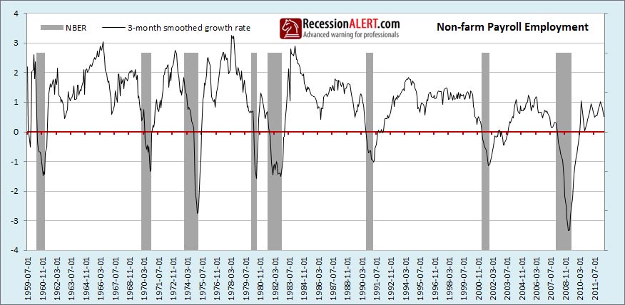
In this instance we have also found the 3-month smoothed growth rate to work the best for signalling recession. This is short enough to be sensitive to rapid changes in employment without whipsawing you will false positives, as shown below:

4. Real Retail Sales

In this instance we have found the 12-month % change (not smoothed) growth rate to work the best for signalling recession. A shorter period results in too many false positives. The growth is shown below:

5. Syndrome Diffusion Index

We have also found 4 thresholds below which each co-incident indicators’ growth shown above must respectively fall to contribute to a recession “syndrome.” They are as follows:

• Industrial Production -1.77%
• Personal Income -0.25%
• Payroll Employment +1.38%
• Retail Sales +0.44%

When each indicator falls below its syndrome trigger, it means nothing on its own and merely counts a vote toward the Syndrome Index. We then take 2 and subtract the number of votes to get a Recession Syndrome Diffusion Index recession dating model. When the index falls below zero (more than 2 systems are below their syndrome triggers) we call recession. The syndrome triggers were obtained from an optimization program to find the values that maximize the Area Under Curve (AUC or ROC) of the resulting recession dating model. These are the values for which the model provides the least amount of false positives, the least amount of false negatives and the highest recession/expansion sorting score. The use of this index considerably enhances the accuracy of the NBER recession dating model we are leading up to:

6. Building the weighted Composite NBER Model

We now have 5 components with which to build a multifactor composite co-incident index:

1. Industrial Production growth (17% weighting)
2. Real personal income growth (31% weighting)
3. Non-farm payrolls growth (30% weighting)
4. Real retail sales growth (12% weighting)
5. Syndrome Diffusion Index (10% weighting)

Using an optimization program, we take these 5 time-series (shown in the 5 charts above) and build them into a weighted composite growth index. The weights the program will assign to each component are those that maximize the performance of the resulting composite index in dating recessions. Thus, they are the weights for which the resulting composite index, when used below zero to trigger recession calls, makes the least amount of false positives, the least amount of false negatives and maximizes the recession/expansion sorting capability of the model. The weights are assigned are shown in brackets above and produce the composite index shown below:

7. Building the Recession Probability Model

We can now take all 6 time series, namely Industrial production, Retail Sales, Employment, Personal Incomes, Syndrome Diffusion Index and the weighted composite and put them through a Probit statistical process to develop a 6-factor recession probability model as shown below:

For timely recession dating using the probability model on its own, you will generally call recession when probability of recession rises above 0.1 (10% chance of recession). This yielded 2 false alarms in the past. To use a threshold that has never resulted in a false alarm, use 0.4 (40%) although you sacrifice 1-2 months lead time for this privilege… RecessionALERT subscribers have all the charts shown in this research note updated each week in their regular report.

*Editor's note: Update 23 Jul 2012 with new content below:*

8. Testing model resilience

The recession model weighted composite we built in section-6 was based on an optimization running through the entire data set, namely 1959 through to July 2012. As part of normal rigorous statistical testing we need to ensure that this optimization was not a lucky random configuration and that the 4 co-incident indicators in an optimized weighted average model do indeed consistently reflect behavior that accurately identifies recessions.

We achieve this by simulating a person sitting in December 1968, right before the second recession shown on all the above charts and attempting the optimization on known co-incident data to that point. We then project that model into the future to present day to see how it would have continued to perform in “out of sample” data. We then re-do the exercise but including data up to just before the 3rd recession. We repeat again including data to the 4th recession, 5th recession and so on until we have 7 vintages of the weighted composite. Basically we simulate what kind of models (vintages) a RecessionALERT researcher would have built through time until present day, with a view to seeing just how varied the results would have been and how well the models performed into the future.

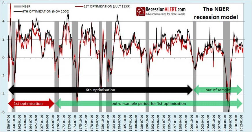
If the results are very varied, or perform poorly into the future (or both) then we conclude the model is at risk of inaccuracy and/or over-optimization. If however, each successive model slightly improves results as more and more data is included into the optimization and each model built over time accurately signals recessions into the future, then we know we have a robust model. The chart below shows two of the models built, namely the very first one built hypothetically in December 1968 (“1st Optimization”) and the 6th one built in November 2000 (“6th Optimization.”) The very last 7th model we built is the one reflected in sections 1 through 7 in this research paper.

We make several remarkable discoveries from the tests. The first model built hypothetically in 1969 using data from 1st July 1959 through to Nov 1969 and encompassing one recession and expansion (red line in above chart) continued to perform remarkably well into the future. Remember, once this model was constituted in November 1969, it was never modified or altered.

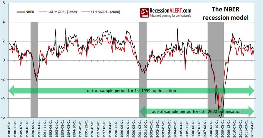
The second important observation is that there is not much difference between the 1st model and the 6th. In fact the correlation coefficient between the two is 0.90. Although the two models differed, they differed less around business cycle turning points than during expansion. This means their differences would not have had much impact on dating accuracy as shown in the zoomed view below:

The third remarkable observation is that all 7 models built just before the start of each NBER recession have the same two characteristics described above – they all performed well into the future (out of sample data) and they all did not differ that much when it came to detecting business cycle turning points (starts and ends of recessions.) The charts below show all 7 model vintages built over time, with the maximum readings, minimum readings as well as the average of all 7 readings for each month. You will also note that the average of all 7 models hugs the maximum high watermark rather than sitting centrally between the low and high watermark – suggesting the low readings are outliers of all 7 vintage models.

An obviously interesting point to make is that even the lowest current reading of all 7 vintage optimization models is not currently flagging recession. In other words, the most pessimistic reading of all 7 models is currently not flagging recession.

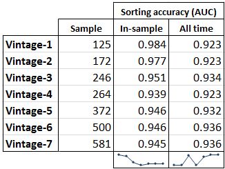
The visual inspection of the above charts leads us to believe that although the time-series of each model may differ, these differences are small at turning points. But we should rather confirm this by looking at the “area under the curve” (AUC or sometimes referred to as ROC) scores for each model, where we rank their ability to sort all months correctly between expansion and recession. A model that perfectly sorts all 580 months into proper buckets for expansion and recession scores a 1.0 in this method. The results are shown in the table below and they indeed confirm that turning point identification accuracy among all model vintages is highly comparable. We see that the more months included in the sample for the models’ optimization, the more accurate the model becomes over the whole time period. But there is not much difference between the models in relative terms.

We can thus safely conclude that the weighted average model we developed through optimization with the 4 specified “NBER co-incident indicators” plus the diffusion index, does not owe its accuracy to random luck or over optimization and each successive model we build over time with more in-sample data is likely to continue to perform well into the future and improve overall accuracy.

9. Another perspective

Doug Short independently published his own detailed analysis within minutes of us publishing this note. For another insightful examination of the NBER co-incident indicators that come to the same conclusions, but taken from a different angle, see Doug Shorts’ “The Big Four Economic Indicators: What They’re Telling Us about a Recession.“.

Source: Recession Alert